- While investments in defensive equity strategies have surged since the GFC, the key question is how to increase upside participation while maintaining downside protection.
- Minimum variance portfolios have long formed the basis of defensive equity strategies, but by enhancing them with dynamic components, they can provide better returns and protection.
- A signal comprising of macroeconomic, valuation and momentum allows a dynamic strategy to increase its participation in bull markets without a deterioration of asymmetry and without an increase in turnover or transaction costs.
Overview
The first reference to Low Risk investing dates back to the 1970s and the work carried out by Haugen and Heinz1, who noticed that portfolios composed of low volatility stocks consistently outperformed their high volatility counterparts. This Low Volatility anomaly later became the basis of an investment style commonly referred to as defensive equities, characterised by beta to a capital weighted benchmark of between 0.6 and 0.7, and a positive alpha of 2-3% annualised.
Investments in defensive equities surged following the Great Financial Crisis (2007 to 2009). Interestingly though, the timing of such a shift into defensive mode has not been beneficial to latecomers in this space. In strongly rising markets, investors who focus on low beta are bound to be playing a catch-up game.
One can illustrate the problem in the following hypothetical example. Assume you have a strong persistent alpha of 3% annualised in a Low Volatility investment strategy exhibiting a beta of 0.7 to a capitalisation weighted market. If equity market returns are not strong, you get to benefit from your alpha by outperforming the benchmark – a 5% annual market return will let you harvest 1.5% of outperformance. However, in strongly rising markets your alpha will not be sufficient to offset your beta drag. A 30% year in the market will see your strategy underperforming by 6%.
Inevitably, the question arises on whether one can manage the relative risk of a defensive strategy in bull markets while retaining a strong level of protection in down markets.
To Time or Not to Time – That is the Question
The question of timing financial markets or risk premia has been central to investment discussions for more than 50 years. Initial claims of market efficiency from proponents of buy-and-hold investments have slowly been brushed aside by overwhelming evidence to the contrary. By the early 1990s, valuation as the tool to time equity markets over a longer horizon had become mainstream2. And, following deep global recessions in the 2000s, macroeconomic indicators have become indispensable in determining positioning for many market players. Nowcasters for growth, inflation and market stress, along with valuation, have proven to be effective timing tools beyond just equity markets, working well for alternative risk premia too3. The discussion over the timing of equity factor performance has also shifted over the years from a strong position of “collecting equity premia” with no dynamic components to acknowledging that equity premia performance varies significantly over time and can be predicted to a certain extent. In fact, both academic studies and practitioner research indicate that factor valuation and factor momentum are useful tools for equity factor timing4.
Performance of a Minimum Variance Equity Portfolio and Opportunities for Efficient Timing
One of the popular ways to implement a defensive equity strategy is by constructing a long-only minimum variance portfolio. This should not come as a surprise as minimum variance portfolios are optimal according to modern portfolio theory when we have no reliable information about the expected returns of individual securities5.
Synthetic relative performance of a simple minimum variance portfolio constructed using the MSCI World universe with simple diversification constraints and transaction cost penalties (a feature that aims to account for transaction costs, acknowledging the turnover cannot be unlimited) is shown in Figure 1 (blue line, left axis). In a backtest, a simple minimum variance strategy with an average beta of 0.6 outperformed the MSCI World benchmark by nearly 50% over the past 20 years while showing strong cyclicality. As expected, periods of underperformance coincided with strongly rallying equity markets.

Our proprietary nowcasters demonstrate that macro data can be useful to distinguish periods of under- and outperformance of a minimum variance strategy

Figure 1 also shows our proprietary growth and inflation nowcasters, indicators developed by Unigestion to measure the state of the macroeconomic environment at a given point in time. The nowcasters demonstrate that macro data can be useful to distinguish periods of under- and outperformance of a minimum variance strategy. Another useful macro component is a market stress nowcaster, shown in Figure 2. As expected, high values of the market stress nowcaster coincide with periods of outperformance for a minimum variance strategy.
In Figure 3, we show relative valuation of equities vs bonds in a cross-section of relevant risk premia. It is well known that low volatility stocks exhibit bond-like properties. When bonds are expensive vs equities we would expect bonds and, therefore, low volatility stocks to underperform. In Figure 3, we can observe that local maxima of bond relative valuation precede the periods of underperformance of a minimum variance strategy.
Figure 1: Relative Synthetic Performance of a Minimum Variance Strategy and Growth and Inflation Nowcasters
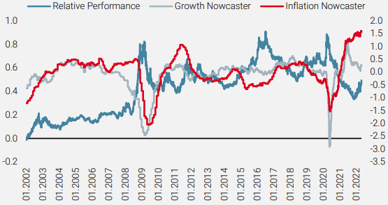
Source: Bloomberg, Unigestion. Data as at April 2022. Relative synthetic performance of a minimum variance strategy vs MSCI World capital weighted benchmark (left axis). Growth and inflation nowcasters (right axis) are negatively correlated with minimum variance excess return.
Figure 2: Relative Synthetic Performance of a Minimum Variance Strategy and Market Stress Nowcaster
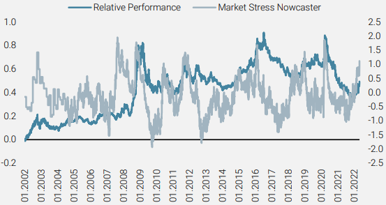
Source: Bloomberg, Unigestion. Data as at April 2022. Relative synthetic performance of a minimum variance strategy vs MSCI World capital weighted benchmark (left axis). Market stress nowcaster (right axis) is positively correlated with minimum variance excess return.
Figure 3: Relative Synthetic Performance of a Minimum Variance Strategy and Relative Valuation of Equities vs Bonds
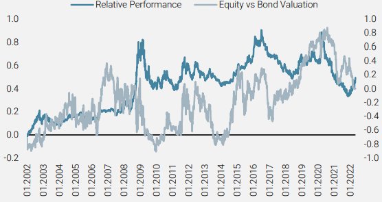
Source: Bloomberg, Unigestion. Data as at April 2022. Relative synthetic performance of a minimum variance strategy vs MSCI World capital weighted benchmark (left axis). Relative valuation of equities vs bonds (right axis). Negative values for relatively expensive equities, positive for relatively expensive bonds.
The large tracking errors in low risk investing seen following strong outperformance or before steep declines is a function of the negative correlation of volatility and equity market returns
In Low Risk investing, large realised tracking errors (TE) are typically observed after periods of strong outperformance and preceding a steep decline. This observation is supported by a well-known stylised fact of a negative correlation of volatility and equity market returns (the main reason for a negative skew in market return distributions).
In Figure 4, we can see the relative performance of a minimum variance strategy vs the MSCI World index and the corresponding TE (over 3 months, annualised, right axis). The correlation of TE with the future relative 3-month return of the MSCI MinVol is -0.28 over the entire period.
It is important to combine a mean-reversion signal with a momentum signal. As is customary for many equity factors, positive short-term momentum is indicative of the continued outperformance of a minimum variance strategy.
Figure 4: Relative Synthetic Performance of a Minimum Variance Strategy and Tracking Error
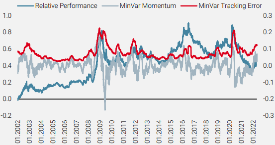
Source: Bloomberg, Unigestion. Data as at April 2022. Relative synthetic performance of a minimum variance strategy vs MSCI World capital weighted benchmark (left axis). 3-month momentum and tracking error of a minimum variance strategy (right axis). Negative momentum and a high TE are predictive of underperformance of a minimum variance portfolio.
What is Your Horizon?
It is not by accident that we talked about a 3-month horizon in the previous section. Whenever a dynamic strategy is discussed and when designing the signal, it is important to take into account a realistic rebalancing schedule. While futures-based strategies can be rebalanced with a daily or weekly frequency, transaction costs of cash equity trading limit most asset managers to more conservative rebalancing schedules. In these circumstances, we find that a horizon of between one and three months is meaningful. This horizon then determines how we evaluate signal performance.
While the signal’s components are weak on their own, their combination produces a strongly significant indicator
Putting It All Together in an Ensemble
We can now put together all timing signals mentioned in this paper so far. We adjust the signal components to indicate aggressive positioning for the high values of each component. As mentioned previously, growth, inflation and market stress are based on our proprietary global nowcaster time series, relying strongly on their diffusion index parts. A proprietary valuation signal is based on the relative valuations of equities and bonds in a cross-section of relevant risk premia. This signal is more responsive than time-series-based valuation signals. The use of bond data is a reflection of the bond-like properties of risk managed equities. Momentum and mean reversion signals are derived from the 3-month relative performance and TE of a minimum variance synthetic strategy with respect to the capital weighted benchmark.
Over the past 20 years, signal components have shown statistically significant correlations with the 1-month forward excess return of a minimum variance strategy. However, they are not sufficiently reliable to use individually. Having said that, combining these weak signals in an ensemble produces a strongly significant indicator. When doing so, correlation with the 3-month forward excess return is even stronger at -0.32.
Table 1: One-month Correlations

Source: Bloomberg, Unigestion. Data as at April 2022.
Figure 5 illustrates a 3-year rolling correlation of the combined signal with 1-month and 3-month excess returns and shows that the signal is useful over most of the history.
Figure 5: Three-Year Rolling Correlations of the Combined Signals
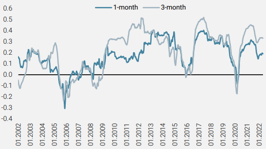
Source: Bloomberg, Unigestion. Data as at April 2022. 3-year rolling correlation of the combined signal with 1-month and 3-month forward excess returns of a minimum variance strategy vs MSCI World benchmark.
Another way to access the signal’s behaviour is to evaluate hit ratios of the minimum variance strategy’s relative returns at various levels of the signal. Despite strong cumulative outperformance over 20 years, the minimum variance approach shows higher 1-month returns than a capital weighted benchmark only 49.5% of the time. The dynamic signal is expected to add value if the hit ratio becomes higher when this signal indicates defensive positioning and lower when the signal shows a risk-on state. In Table 2, we separate each signal component into defensive and aggressive positioning. We see that each signal component improves the frequency of minimum variance outperformance in defensive states and indicates that it is more beneficial to be closer to the benchmark in aggressive states.
Table 2: Defensive and Aggressive Split of Signal Components
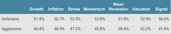
Source: Bloomberg, Unigestion. Data as at April 2022.
How to Implement It
While discussing implementation details is outside the scope of this paper, we point out two potential avenues for making use of the above signal in practice. The first involves using index futures in addition to holding a Low Risk strategy. Ease of implementation and low transaction costs are advantages of this approach. In the cash equities space, an implementation that uses both variance and square of tracking error penalty terms in the objective function is appealing (see Appendix). The signal can be used as a trade-off coefficient between TE2 and variance terms.
When we are in fully defensive mode we minimise variance, i.e. tracking error to cash. When the signal shows a more aggressive stance our target is a combination of the benchmark and cash. Scaling the signal appropriately, we can retain defensive properties with beta of our target always smaller than 1, even in the most aggressive position, while keeping turnover and transaction costs at the same level as for a minimum variance strategy.
Figure 6: Relative Synthetic Performance of a Minimum Variance and a Dynamic Strategy
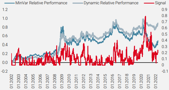
Source: Bloomberg, Unigestion. Data as at April 2022. Relative synthetic performance of a minimum variance strategy and a dynamic strategy vs MSCI World capital weighted benchmark (left axis). Dynamic signal is shown on the right axis on a scale from zero (fully defensive) to one (risk-on).
Table 3: Minimum Variance vs Dynamic
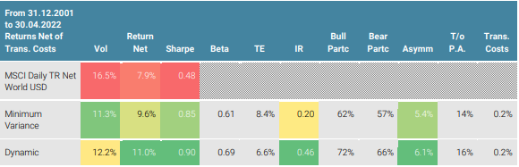
Source: Bloomberg, Unigestion. Data as at April 2022.
The variability in performance of a minimum variance strategy and its structural vulnerability in strongly rising markets calls for a dynamic approach.
Conclusion
The variability in performance of a minimum variance strategy and its structural vulnerability in strongly rising markets calls for a dynamic approach where the beta of the strategy needs to be increased when markets are rallying. A signal comprising of macroeconomic, valuation and momentum components allows a dynamic strategy to increase its participation in bull markets without a deterioration of asymmetry and without an increase in turnover or transaction costs compared to a basic minimum variance strategy.
1Haugen R. A. and Heinz A. J. “Risk and Rate of Return on Financial Assets: Some Old Wine in New Bottles” Journal of Financial and Quantitative Analysis vol. 10, pp 775-784, 1975
2Cochrane J.H. “Presidential Address: Discount Rates” Journal of Finance vol. 66, pp 1047-1108, 2011
3Baig S., Lee J., Teiletche J. “An Introduction to Unigestion’s Macro Nowcasters: Real-Time Tracking of the Economy” Unigestion Research, June 2022
4Arnott R. D., Clements M., Kalesnik V., Linnainmaa J. T. “Factor Momentum” SSRN, March 2021.
5Dubikovskyy V. and Susinno G. “Solving the Rebalancing Premium Puzzle” Risk-Based and Factor Investing. Edited by Jurczenko E. Elsevier, pp 228-246, 2015
Appendix: Minimising Variance and Tracking Error at the Same Time
Let’s write out what we want to minimise. Assume we put a scale parameter λ in front of the variance term. We get:
„λ“ σ_p^2+〖TE〗^2=“λ“ σ_p^2+σ_p^2+σ_b^2-2ρσ_p σ_b
where σp is the portfolio volatility, TE is the tracking error to the benchmark, σb is the benchmark volatility and ρ is the correlation between the portfolio and the benchmark. We also introduce β as the portfolio beta.
Let’s regroup the terms of what we optimise:
„λ“ σ_p^2+〖TE〗^2=(„λ+1)“ (σ_p^2-(2ρσ_p σ_b)/(λ+1)+(σ_b^2)/(λ+1)^2 )+(λσ_b^2)/(λ+1)
We note that the last term does not depend on portfolio weight (indeed only σp and ρ do). In a minimisation problem we need to set partial derivatives with respect to asset weights to zero. Derivatives of the last term are zero. Thus the problem is equivalent to minimising the term in the brackets.
Let’s ask ourselves: what is the expression for the tracking error (TEpart) between our portfolio and a specific combination of the benchmark and cash (we take 1/(λ+1) of benchmark and λ/(λ+1) of cash)? We find:
〖TE〗_part^2=σ_p^2-(2ρσ_p σ_b)/(λ+1)+(σ_b^2)/(λ+1)^2
Note that the correlation between a portfolio and the benchmark and a portfolio and any non-zero cash/benchmark combination is the same.
We notice that minimisation of variance and TE to the benchmark is equivalent to minimisation of TE to a weighted combination of the benchmark and cash.
Important information
Past performance is no guide to the future, the value of investments, and the income from them change frequently, may fall as well as rise, there is no guarantee that your initial investment will be returned. This document has been prepared for your information only and must not be distributed, published, reproduced or disclosed by recipients to any other person. It is neither directed to, nor intended for distribution or use by, any person or entity who is a citizen or resident of, or domiciled or located in, any locality, state, country or jurisdiction where such distribution, publication, availability or use would be contrary to law or regulation.
This is a promotional statement of our investment philosophy and services only in relation to the subject matter of this presentation. It constitutes neither investment advice nor recommendation. This document represents no offer, solicitation or suggestion of suitability to subscribe in the investment vehicles to which it refers. Any such offer to sell or solicitation of an offer to purchase shall be made only by formal offering documents, which include, among others, a confidential offering memorandum, limited partnership agreement (if applicable), investment management agreement (if applicable), operating agreement (if applicable), and related subscription documents (if applicable). Please contact your professional adviser/consultant before making an investment decision.
Where possible we aim to disclose the material risks pertinent to this document, and as such these should be noted on the individual document pages. The views expressed in this document do not purport to be a complete description of the securities, markets and developments referred to in it. Reference to specific securities should not be considered a recommendation to buy or sell. Unigestion maintains the right to delete or modify information without prior notice. Unigestion has the ability in its sole discretion to change the strategies described herein.
Investors shall conduct their own analysis of the risks (including any legal, regulatory, tax or other consequences) associated with an investment and should seek independent professional advice. Some of the investment strategies described or alluded to herein may be construed as high risk and not readily realisable investments, which may experience substantial and sudden losses including total loss of investment. These are not suitable for all types of investors.
To the extent that this report contains statements about the future, such statements are forward-looking and subject to a number of risks and uncertainties, including, but not limited to, the impact of competitive products, market acceptance risks and other risks. Actual results could differ materially from those in the forward-looking statements. As such, forward looking statements should not be relied upon for future returns. Targeted returns reflect subjective determinations by Unigestion based on a variety of factors, including, among others, internal modeling, investment strategy, prior performance of similar products (if any), volatility measures, risk tolerance and market conditions. Targeted returns are not intended to be actual performance and should not be relied upon as an indication of actual or future performance.
No separate verification has been made as to the accuracy or completeness of the information herein. Data and graphical information herein are for information only and may have been derived from third party sources. Unigestion takes reasonable steps to verify, but does not guarantee, the accuracy and completeness of information from third party sources. As a result, no representation or warranty, expressed or implied, is or will be made by Unigestion in this respect and no responsibility or liability is or will be accepted. All information provided here is subject to change without notice. It should only be considered current as of the date of publication without regard to the date on which you may access the information. Rates of exchange may cause the value of investments to go up or down. An investment with Unigestion, like all investments, contains risks, including total loss for the investor.
Legal Entities Disseminating This Document
UNITED KINGDOM
This material is disseminated in the United Kingdom by Unigestion (UK) Ltd., which is authorized and regulated by the Financial Conduct Authority („FCA“). This information is intended only for professional clients and eligible counterparties, as defined in MiFID directive and has therefore not been adapted to retail clients.
UNITED STATES
This material is disseminated in the United States by Unigestion (UK) Ltd., which is registered as an investment adviser with the U.S. Securities and Exchange Commission (“SEC”). All inquiries from investors present in the United States should be directed to Clients@unigestion.com at Unigestion (UK) Ltd. This information is intended only for institutional clients and qualified purchasers as defined by the SEC and has therefore not been adapted to retail clients.
EUROPEAN UNION
This material is disseminated in the European Union by Unigestion Asset Management (France) SA which is authorized and regulated by the French “Autorité des Marchés Financiers” („AMF“).
This information is intended only for professional clients and eligible counterparties, as defined in the MiFID directive and has therefore not been adapted to retail clients.
CANADA
This material is disseminated in Canada by Unigestion Asset Management (Canada) Inc. which is registered as a portfolio manager and/or exempt market dealer in nine provinces across Canada and also as an investment fund manager in Ontario, Quebec and Newfoundland & Labrador. Its principal regulator is the Ontario Securities Commission („OSC“). This material may also be distributed by Unigestion SA which has an international advisor exemption in Quebec, Saskatchewan and Ontario. Unigestion SA’s assets are situated outside of Canada and, as such, there may be difficulty enforcing legal rights against it.
SWITZERLAND
This material is disseminated in Switzerland by Unigestion SA which is authorized and regulated by the Swiss Financial Market Supervisory Authority („FINMA“).
Document issued July 2022.