The risky asymmetry of low bond yields

Introduction

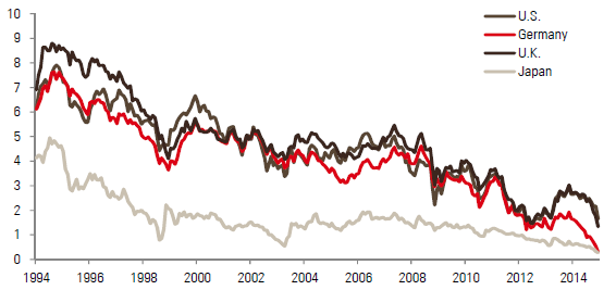
As everyone knows, we are living in a world of historically low interest rates. In the US, ten-year yields have not been this low in the past 50 years (Figure 1). In the rest of the developed world, most rates are below 2%, converging towards Japanese bond yields (Figure 2).

Figure 1 – US ten-year Treasury yield (%)

 

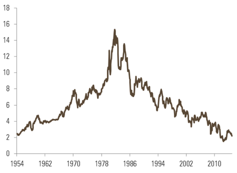
Figure 2 –Ten-year government yields (%) in major developed economies

 

As bond yields are reasonable forecasters of future bond returns – at least over long horizons – investors in traditional multi-asset solutions are facing the possibility of inadequate returns. In this paper, we stress another negative implication of low bond yields that relates to portfolio construction.

One of the basic premises of multi-asset solutions is to combine assets that provide growth potential – typically equities – with diversifying assets such as bonds, which are supposed to generate higher relative returns while equities suffer in certain environments, such as economic recessions or market shocks. The problem with current low bond yields is that the potential for a further decline in yields is lower because rates cannot fall much further, limiting the potential for their prices to increase and hence provide protection during such shocks.

In this paper, we show how this dislocation, mainly driven by exceptional central bank policies (together with the exceptional situation on inflation), leads to an unusual negative skew in the distribution of bond returns. On that basis, we suggest ways to deal with this dislocation in an asset allocation framework.

(Almost) zero interest rates and negative skewness: a less well-known Japanese experience

In a recent research note, Morris (2014) points out an interesting characteristic on the distribution of Japanese government bonds (JGBs): they are negatively skewed. In Table 1, we show the volatility and skewness of the distribution of JGB returns and those of other asset classes. The calculations encompass the period covering Japan’s zero interest rate policy, which started in 1999, and was followed by QE (quantitative easing) in 2001 and a long period of almost-zero short-term interest rates that the Bank of Japan has pursued since then (with a short exception between 2006 and 2008 when it raised rates by 50 basis points).

We can see that this negative skewness is not observed for other government bonds, whereas it is present for risky asset classes such as equities and high yield bonds. Indeed, it is striking that JGBs show an even more pronounced negative skew than high yield bonds – an asset class that is known for this characteristic.

Table 1 – Skewness (and volatility) of several asset classes returns (April 1999 – December 2014)

	US T-Note	Bund	UK Gilts	JGB	S&P 500	US High Yield
Volatility	6.1%	5.2%	5.9%	3.1%	15.3%	11.3%
Skewness	0.25	0.13	0.27	-0.96	-0.57	-0.94

 

Sources: Bloomberg, Government bonds and equity indices are based on futures contracts, while the high yield index is the Barclays US Corporate index. Returns used in calculating volatility and skewness are in excess of cash for government bonds and equities, and in excess of government bonds (duration-adjusted) for high yield.

Skewness and investments

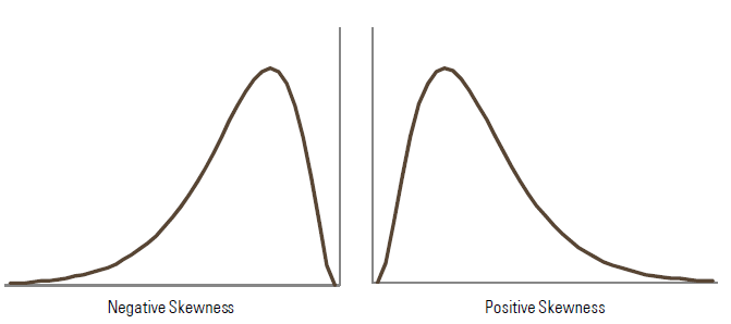
What is skewness? In statistical terms, it is a measure of the asymmetry of the probability distribution of a variable around its mean. Skewness is equal to zero for a symmetric distribution such as the normal (Gaussian) distribution, but more generally, it can be positive or negative.

As Figure 3 shows, negatively skewed distributions are characterised by most of the distribution being concentrated on the right-hand part, where the values are higher than the mean. At the same time, fewer of the observations can be found in the fairly long left-hand tail, where values are lower than the mean.

In simple terms, with a negative skew the realisations of the random variable frequently turn out to be numbers slightly higher than the mean and, less frequently, numbers lower than the mean and very large in absolute terms (i.e. big losses for financial returns distributions). The opposite is true for positive skewness.

Figure 3 –Distributions with negative and positive skewness

 

Skewness can be identified in a number of economic or financial situations. A well-known example of a positively skewed distribution concerns wages. Many countries have implemented a minimum wage and a significant proportion of people earn close to this minimum wage while few earn significantly more. In other words, the distribution of wages is characterised by a large mass at low levels and a long thin right tail. Another example is the lottery, where the great majority of people win nothing while a very small number win a lot, leading to a similar distribution pattern.

In investing, return distributions with a positive skew are fairly rare. As Table 1 shows, over the long term, developed market government bonds are one example. Another well-known example is cross-asset trend-following strategies, such as those pursued by CTA managers.

Negative skewness is much more common, which is unfortunate for investors. Negative asymmetry in return distributions often characterises risky strategies. A well-known example is short volatility strategies in equity markets. For instance, consider an investor who every month sells 10% out-of-the-money puts on the S&P 500 with a monthly horizon. The investor collects the put premia each month, providing a regular return, with the exception of months in which the S&P 500 loses more than 10%, in which case the put is in-the-money and the investor could face a large loss. This means that the return distribution is characterised by many low positive returns corresponding to the months in which premia are collected and put options are not exercised, and a small number of large monthly losses when the equity market declines significantly.

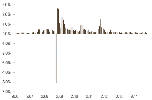
Figure 4 shows the history of such a strategy’s monthly returns from 2006 to 2014 for the S&P 500. The returns have been consistently positive over that period, with very low volatility (2.4% annualised) with one exception. In October 2008, the strategy lost more than 5% as the S&P 500 fell by almost 17%. This loss represented seven times the standard deviation of monthly returns – an event that has an almost-zero probability for a Gaussian-normal distribution.

The skewness of the distribution of returns is -3.7, a high figure in absolute terms, showing that for this kind of strategy, skewness is a better measure of the risk than volatility.

Figure 4 –A highly asymmetric strategy: monthly returns from selling 10% out-of-the-money puts on the S&P 500

 

Credit is another example of an asset class with a negative skew, as shown by the figures for high yield bonds in Table 1. With a bond that may default, an investor who holds to maturity will approximately receive the yield – and hence a positive return – unless the issuer defaults in which case they could suffer a significant loss and even loose all of their capital if the recovery rate is zero. Such a distribution exhibits significant skewness.1

Skewness as a risk measure

Skewness can, therefore, be used to identify asymmetric trades and, particularly for strategies with a negative skew, can be deemed as a sensible risk measure.2 In a recent paper, Lempérière et al. (2014) shows that skewness is much more useful than volatility in explaining differences in risk premia (i.e. average excess return) between assets in most universes. Indeed, while the relationship between excess returns and volatility is unclear, there is a strong correlation with skewness: assets with a large negative skew post the largest excess returns.

Table 1 shows an asset’s risk ranking relative to others based on volatility or skewness: the two measures do not yield the same rankings. While JGBs for example, appear the least risky in terms of volatility, they display the most negative skewness.

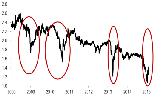
The risk of JGBs can be shown in other ways. For instance, Figure 5 shows that there have been several violent short- term movements in the yield on 30-year JGBs since the Great Financial Crisis began.

Figure 5 – Thirty-year Japanese bond yields (%)

 

When bond yields are at a floor: setting the stage for asymmetry in returns

While skewness seems an attractive risk measure for equities and credit, what is the rationale for using it for government bonds? We argue, as illustrated by the Japanese experience, that when yields are approaching 0%, volatility is no longer a relevant risk measure for government bonds.3 Critical to this assertion is that we assume there is a lower boundary (floor) that yields cannot breach or, at the very least, are unlikely to breach.

Until very recently, almost everyone would have put this minimum at 0%. But the world has changed and it is now clear that interest rates can fall below zero for many currencies and issuers.4

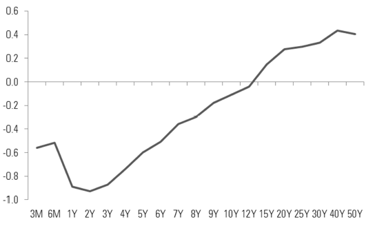
This is most pronounced in Switzerland. After the Swiss National Bank’s decision to abandon the Swiss franc’s ceiling to the euro and to lower its Libor target further into negative territory, interest rates became negative for all bonds with tenor of up to 12 years (Figure 6).

Figure 6 –Interest rate curve in Switzerland (as at 20 January 2015, %)

 

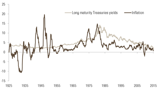
The negative yields mean that investors holding these bonds to maturity accept that they will lose money, at least on a nominal basis. It is noticeable that in Japan, such a situation has only happened very recently and for bonds with short maturities. The US has never experienced periods of negative yields, even during episodes of deflation, such as the 1930s and 1950s (Figure 7).

Figure 7 – US long-term yield (%, over ten years) and US inflation (%): a long-term view

 

Quantifying the asymmetry of risk assuming bond yields have a floor

If we start from the principle that bond yields do have a lower boundary, then the potential of asymmetric distribution for bond returns exists. The total return of a bond TR, can be approximated as follows:

TR ≈  −D × ∆r +  rO

D is the initial duration, ∆r is the change in bond yield over the period and rO is the initial yield. If we set a floor at 0%, then the potential movement in bond yields ∆r ranges from −rO to +∞. Applying the total return equation above, this implies that the returns can range between −∞ and +(D + 1)rO. So, while losses are potentially unlimited, positive returns show a boundary.

As an extreme case, if the initial yield is at the floor i.e. rO = 0, then the investor can at best have a 0% return, but will probably suffer losses.

How can we quantify this asymmetric characteristic more precisely? The problem is that empirical measures based on historical data are not useful because this kind of asymmetric risk is more about what could happen in the future than looking at what did happen in the past.5 This means that ex-ante corrections for skewness measures are required. Given that the duration of a bond increases when its yield falls, computing the volatility of bond prices as the product of bond yield volatility and current duration will lead to higher volatility at low interest rates. However, this correction is modest at best.6 Neither are traditional interest rate risk models able to cope with low interest rates. In particular, the lognormal process is, by definition, unable to cope with zero interest rates and implies that bond volatility vanishes as interest rates approach zero.7

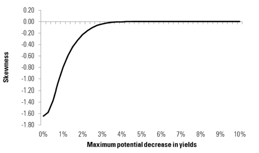
We suggest quantifying the skewness implied by the floor through simulations8. We assume that an investor holds a bond with a duration of eight years. The volatility of its yield is presumed to be 1%, which is typical for ten-year interest rates over the long term. We simulate changes in the yield to be drawn from a normal distribution with zero drift, but we set a floor on bond yields, hence capping the maximum reduction in yields that is achievable. If the starting bond yield is well above the floor, then the potential decrease in yield is large. On the contrary, if yields are already low and close to the floor, their maximum potential fall is small. We performed 10,000 such simulations.

Figure 8 shows the resulting median skewness across the simulations that we performed.9 We see that when bond  yields start from low levels, hence have limited potential to fall further, the skew is strongly negative. This clearly illustrates the fundamental asymmetry involved in buying bonds with low yields.

Based on our hypothetical simulations and the complementary calculations in the Appendix, we can estimate that, if the bond floor is set at 0%, the skew problem arises as soon as bond yields are below 3%.

Figure 8 – Theoretical skewness of bond returns conditional on maximum potential fall in yields

 

It is also important to note that in contrast to other negatively skewed strategies, the returns associated with lower bond yields also worsen, while they are positive for volatility selling or credit spreads. This indicates the risk-reward trade-off becomes highly unattractive at low yields.

Asset allocation implications for investors

The negative skew of bond returns at low yields has a number of implications for investors.

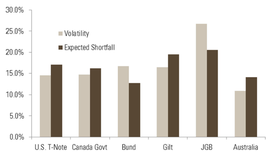
First, the investors need to adapt the way they allocate within their bond portfolio and consider the implications of negative asymmetry in their portfolio construction. Starting from a universe of the most liquid ten-year bond futures, Figure 9 shows the output of two different risk-based allocation mechanisms, where allocated weights are proportional to the inverse of the two risk measures: implied volatility and a generalised risk measure. The latter is a measure of the projected expected shortfall i.e. the expected average loss in the 5% of worst cases over the coming year and incorporates a number of dimensions of risk: valuation through carry, volatility and asymmetry. As shown by the lower weight of JGBs, we see that the allocation can differ significantly depending on how we define risk. We would strongly argue against using volatility as the allocation criterion as it can lead to an underestimation of risk.

Figure  9 – Risk-based allocations  in a sovereign bond portfolio based on volatility and  generalised  expected shortfall  (9 February 2015)

 

Second, there is the more general question of whether to hold sovereign bonds at all in a portfolio. A simple solution could be to hold no bonds, but depending on the objectives of the client, this may or may not be the right decision. In a deflationary world, sovereign bonds can be among the best-performing assets, as has been the case in Japan. High- quality corporate bonds can also perform well in such an environment. At the other end of credit, we would not recommend high yield bonds as the liquidity in these markets has severely deteriorated. Investors should also seek other sources of return, whether through broad geographical diversification in their bond portfolios, low-volatility equities or the addition of alternative risk premia such as momentum or long-short carry strategies. Private debt instruments also have attractive features as the constraints on lending possibilities from banks are creating supply and demand imbalances in favour of investors that have the ability and willingness to lock their capital in exchange of an attractive risk-adjusted level of income.

Beyond their role as a source of income, bonds are normally also used within asset allocation for the buffer they provide during hard times for other asset classes – in particular growth assets that are suffering during recessions, inflationary shocks or episodes of market stress. Given the current level of yields, investors should accordingly diversify their sources of protection.

Cross-asset momentum (trend-following) strategies, such as those used by CTA managers, could be an attractive solution. Meanwhile, overreaction by the markets can enable investors to opportunistically hedge in areas where the cost of protection seems limited relative to the reward if the negative event they are designed to protect against arises.

In total, bond yields being close to their potential floor is a cause of concern for investors. As well as the reduced income that bonds are providing, their ability to protect a balanced portfolio against shocks to growth-orientated assets such as equities has diminished. So now more than ever, multi-asset investors need to exploit flexible, risk-based solutions, in which risk has a broader meaning than volatility alone and returns are sourced from a wider opportunity set. Furthermore, the optimal allocation is likely to change over time and frequent re-assessment of the strategy is necessary.

This paper has illustrated that for the bond part, such a review may be guided by the difference between the current yield and what the investor estimates as the floor to get a proxy for the negative skewness.

References

Douady R. (2013), The Volatility of Low Rates, Riskdata.

Getmanski M., Lo A., and Makarov I. (2004), An econometric model of serial correlation and illiquidity in hedge fund returns, Journal of Financial Economics, 74, pp. 529–609.

Ilmanen A. (2012), Do Financial Markets Reward Buying or Selling Insurance and Lottery Tickets?, Financial Analysts Journal, 68(5), pp. 26-36.

Lempérière Y., Deremble C., Nguyen T-T., Seager P., Potters M., Bouchaud J-P. (2014), Risk Premia: Asymmetric Tail  Risks and Excess Returns, SSRN n°2502743.

Martellini L., Milhau V., and Tarelli A. (2014), Towards Conditional Risk Parity — Improving Risk Budgeting Techniques in Changing Economic Environments, EDHEC working paper.

Merton R. (1974), On the Pricing of Corporate Debt: The Risk Structure of Interest Rates, Journal of Finance, 29(2), pp. 449-470.

Morris T. (2014), The Tortoise and the Hare, Nomura.

Pender J. (2015), The Truncated Normal Distribution: Applications to Queues with Impatient Customers, Operations Research Letters.

Appendix: analytical approximation on the impact of a yield’s floor on skewness

In the main text, we quantified the effects of a lower bound on bond yields on skewed distribution by using simulations. In this appendix, we take an analytical approach, which is slightly more complex but provides us with some further general insights into skewed distributions. In doing so, we assume that changes in bond yields are distributed according to a truncated normal distribution, i.e. a normal distribution that is bounded on one or both sides of the distribution.

Let ∆rmin be the lowest achievable change in bond yield (centred and standardised by bond yield changes, mean and volatility respectively). It ranges from −∞ if there is no constraint (a very unrealistic case) to zero if yields cannot decrease further. By letting ∆rmin vary, we can illustrate the impact on the skewness of the distribution. At the other side of the spectrum, we assume that interest rates can always increase to infinity.

 

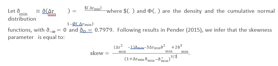
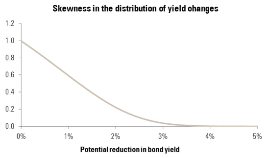
If there is limited constraint in the potential reduction of bond yields (i.e. ∆rmin is very negative), then the skew is equal to zero as ðmin = 0. On the other hand, when bond yield falls are constrained, skewness reaches its highest departure from the Gaussian-normal case. The graph below illustrates this result. Materially, if we assume that the floor on bond yield is 0%, when bond yields are below 3%, their distribution becomes asymmetric. Notice that here we have a positive skew, but we are looking at bond yield changes rather than bond price changes: a positive skew in the distribution of bond yield changes translates into a negative skew for bond price changes.

 

1 There is a strong relationship between the negative skewness of credit and the one of a strategy, selling volatility-on equity. The theoretical model of Merton (1974) shows that being long a corporate bond is equivalent to holding a short position in a put on the underlying firm’s assets (which we can approximate by the equity).

2 While positive skewness in returns can be deemed as favourable, this does not necessarily mean they provide better  payoffs in general than negatively skewed distribution. Quite the contrary, distributions with positive skewness frequently post significant  losses on average, as shown by the lottery example where most people consistently lose money and very few end with a large gain. See Ilmanen (2012) for a discussion.

3 In fact, we believe that volatility is not an appropriate risk measure for bonds in general, as most of them are defaultable and a significant proportion of the market is affected by stale pricing due to illiquidity, which leads to a downward bias in volatility and other risk measures (Getmanski, Lo and Makarov, 2004). This paper focuses on government bonds, which are less affected by these issues, and for which the floor is a more relevant issue for skewness.

4  See Unigestion note “Negative rates: why and how to deal with them?”.

5 Admittedly, one could argue that risk should never be viewed through a rear-view mirror. But our argument is that doing so is even worse in this particular context.

6 See Martellini et al. (2014) for an empirical illustration. Notice that the increased duration effect is also in general accompanied by increased convexity for lower yields.

7 See Douady (2013) for a discussion. The interesting conclusion of this study is that in practice, interest rate volatility has behaved in the past as if the absolute minimum level for a rate was -1% rather than zero.

8  Another possibility, which we describe in the Appendix, is to assume that bond returns follow a truncated normal distribution.

9 The x-axis on Figure 8 represents the maximum fall (in absolute terms) the yield can undergo. The reader can set the floor at the level he thinks is appropriate. For instance, if starting yields are 1% and the floor is set at -1%, then the skewness at a maximum fall in yield of 2% is the relevant value (around -0.2 in this example).

 

---

Important Information

The information and data presented in this page may discuss general market activity or industry trends but is not intended to be relied upon as a forecast, research or investment advice. It is not a financial promotion and represents no offer, solicitation or recommendation of any kind, to invest in the strategies or in the investment vehicles it refers to. Some of the investment strategies described or alluded to herein may be construed as high risk and not readily realisable investments, which may experience substantial and sudden losses including total loss of investment.

The investment views, economic and market opinions or analysis expressed in this page present Unigestion’s judgement as at the date of publication without regard to the date on which you may access the information. There is no guarantee that these views and opinions expressed will be correct nor do they purport to be a complete description of the securities, markets and developments referred to in it. All information provided here is subject to change without notice. To the extent that this page contains statements about the future, such statements are forward-looking and subject to a number of risks and uncertainties, including, but not limited to, the impact of competitive products, market acceptance risks and other risks. 

Data and graphical information herein are for information only and may have been derived from third party sources. Although we believe that the information obtained from public and third party sources to be reliable, we have not independently verified it and we therefore cannot guarantee its accuracy or completeness. As a result, no representation or warranty, expressed or implied, is or will be made by Unigestion in this respect and no responsibility or liability is or will be accepted. Unless otherwise stated, source is Unigestion.

 Past performance is not a guide to future performance. All investments contain risks, including total loss for the investor.